Expected Points

Football is chaotic. Sometimes it looks like something should happen, and then it doesn’t. Over the course of more actions, games, and seasons, these chaotic events tend to balance out towards something that feels more reasonable. Even league winners have days where the ball just doesn’t go in.

We handle this with expected metrics. We have an expectation of an event—an estimate of how likely its different outcomes are—and we use it to better understand what happened, and sometimes predict forward.

For instance, a team might take lots of shots very close to the goal and concede one from 35 yards. For whatever reason, they all miss and the opposition one goes in. It’s probably a good bet that the losing team was better, and the winning team got a bit lucky. It’s a chaotic result.

Expected Goals (xG) measures the probability of each individual shot being scored. We might find that, in our example game, the losing team had an xG value of 2.50 while the winning team had an xG value of 0.01. This is because the losing team had lots of chances that would usually be goals and the winning team had one chance that often isn’t scored. We expect that, from the given chances, the losing team would usually score at least a couple of goals, and the winning team wouldn’t score any.

Obviously, sometimes that doesn’t happen. But, more often than not, when that game plays out that way, the team with 2.50 xG beats the team with 0.01 xG.

This gives us more information about what might happen in the future. If a team is constantly creating chances and they just got unlucky, they’re probably more likely to win their future games than a team not creating any good chances even if they just lost.

And this is exactly how it plays out. When trying to predict future games, Expected Goals are more informative than Actual Goals.

This is well-documented, and is used by clubs and bookmakers for exactly this reason [1].

We can do exactly the same thing with points. A team that was lucky in this way can earn three Actual Points but we may have an expectation—Expected Points (xPts)—that is quite a bit lower. That information helps us understand what happened in that game, and make a better prediction about what might happen in the future.

xG is calculated by looking back at a very large number of shots and asking how often shots like this one were scored. A model takes the details of each shot—where it was taken from, the angle to goal, whether it was a header, how the chance was created, whether it was a penalty—and learns how each of those changes the chance of a goal. A tap-in from six yards might be worth 0.70. A speculative effort from 30 yards might be worth 0.02. A penalty is worth about 0.79, because that is roughly how often they go in.

Add up a team’s xG over a match and you get roughly the number of goals they would usually score from the chances they had.

We use xG from a data provider, so we do not calculate it ourselves. This has pros and cons.

On the plus side, their model is built from far more shots than we could ever collect for one league, it is maintained by people whose job it is to maintain it, and it is the same xG you will see quoted elsewhere, so our numbers line up with what you already know.

On the other hand, we can’t look inside it or change it. If we thought a particular kind of chance was being undervalued, there would be nothing we could do about it. The numbers are also revised after a match, usually with small corrections once the data has been checked, so we collect every match again a day after it is played. Until then, the most recent results on the standings page are marked as provisional.

There are also things that xG doesn’t count. Own goals don’t come from a shot by the scoring team, so they carry no xG. Neither does the dangerous cross that nobody quite got a touch to. xG measures the quality of the chances a team actually had, not every chance it nearly had.

We have several options to calculate xPts, and we consider several factors.

The most intuitive way to think about it is to take every shot in a match and treat it as a biased coin flip that lands on ‘goal’ with the probability of its xG. Flip every coin, count up the goals for each side, and see who won. Do that enough times and you know how often each team would win, draw, and lose with the chances they had. A team’s Expected Points are then three times its chance of winning plus its chance of drawing.

That isn’t the only option. We could add up each team’s xG and assume goals arrive at that average rate, the standard way of modelling goals in football [2]. We could ignore everything except the gap between the two teams’ xG, and learn how often a gap of that size ends in a win. We could even feed all information we have from a match into a machine-learning model and let it work out the rest.

To choose between them, we asked three questions.

Is it right? If a method says a team had a 70% chance of winning, teams in that position should win about 70% of the time.

Is it decisive? A method that says ‘could go either way’ about every match is never badly wrong, but it doesn’t tell us much.

Is it only measuring the chances? xPoints is a useful metric because it isn’t just the result. A method that feeds the result back in defeats the point.

We tested each method on every Scottish Premiership match from 2020/21 to 2025/26, using only that match’s own numbers to predict its result, and repeated everything on the Premier League to check that the patterns held. Each method gets a ranked probability score (RPS)* for how well its probabilities matched what actually happened.

*RPS compares the probabilities given to a home win, a draw, and an away win with what actually happened. It gives more credit for being nearly right (saying draw when the home side won) than for being completely wrong (saying away win), which is why it is the standard way to score football forecasts [3]. Lower is better: 0 would be a perfect forecast every time, and simply using league-wide averages scores about 0.23.

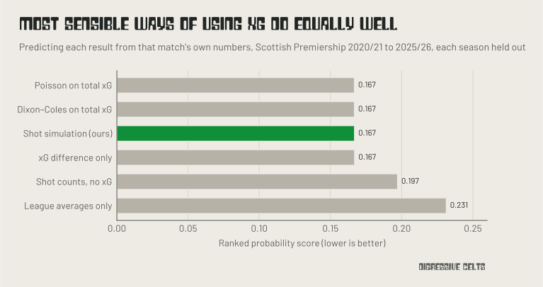
Every sensible way of using xG scored almost exactly the same. Using shots without xG was much worse, and using nothing at all was worse still.

So, why bother with the simulation?

Simply, because it keeps information that alternatives discard. Two teams can both finish a match with 0.80 xG: one from a single penalty, and one from ten 0.10 xG chances. These are not equivalent. The team with the penalty cannot score more than one goal, but is also less likely to not score at all (this can be calculated exactly by plotting out the probability tree). In edge cases where this is relevant, we prefer that this is accounted for.

Machine learning is the interesting one.

When a model is given only the shots from a match, it does marginally better than our more interpretable approaches above. Then, as more information is added—possession, passes, crosses, tackles, clearances, shots on target, saves, cards—the score consistently improves (left of the below graph).

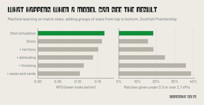
But this is not the model getting better at judging chances. It is instead learning the result. For instance, from shots on target and number of saves, the model has a much better guess at the number of shots that were actually scored. This is a form of data leakage, where the model is able to see information from the result that it shouldn’t and consequently doesn’t learn anything useful.

Each metric here and its relationship with the actual result is adding to this leakage of the result. This stops the model producing a guess at what was most likely to have happened, if luck and noise didn’t factor in, and instead just reproduces the result.

The right of the above graph shows this clearly. The machine learning model produces values much closer to actual results values the more information it has. This is not useful for this task.

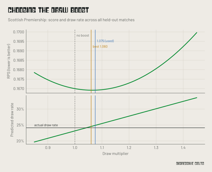
There is one adjustment to make. Treating every shot as an independent observation slightly underestimates draws. In the Scottish Premiership, 24.1% of matches finished level, but the simulation predicted 23.1%. This is because shots are not independent. A team that goes ahead often relaxes, a team that goes behind chases the game, and a rebound only exists because the first shot was saved. Those effects pull matches towards being level a little more often than our first simulation would suggest [4].

So, we scale the chance of a draw up by 7.5%, and take the extra from each side in proportion to their chance of winning. That brings predicted draws to 24.9% without changing who was more likely to win. We checked the sensitivity of this value to ensure our results were robust. We found that the best value for the Scottish Premiership was actually 6% and 9% for the Premier League. The difference between those and 7.5% was never more than 0.14 points over a whole season, so the exact value is unlikely to matter too much. There are more details in Appendix B.

Our final approach, then, works as follows.

For every match, we take each team’s shots and their xG, leaving out own goals. We work out the exact chance of each team scoring any possible number of goals. Instead of actually running the simulation, we do a cool maths trick (outlined in Appendix A) which helps us avoid simulation noise. From the sets of chances for both teams, we get the chance of each possible result. Then, we scale up the draw, and convert the probabilities into Expected Points.

Here’s a real example. Last December, Celtic lost 2–1 at home to Hearts. Celtic had 15 shots worth 1.87 xG. Hearts had 8 worth 0.52, and scored from two small chances, worth 0.11 and 0.02. Celtic’s goal came from a 0.05 chance in the 90th minute.

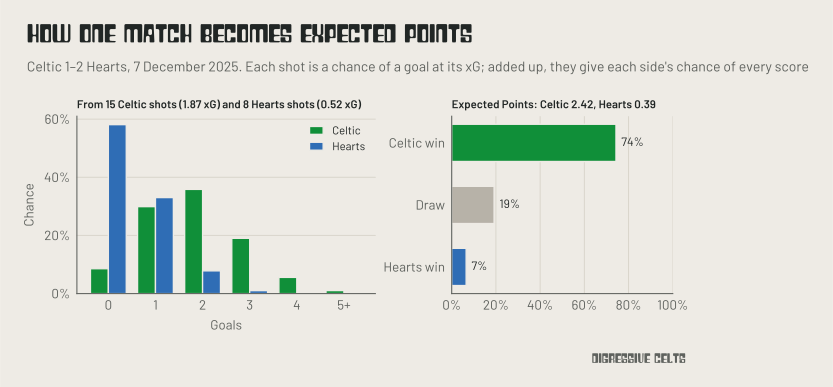
Played out, those chances give Celtic a 74% chance of winning, 19% of a draw, and 7% of losing. That is 2.42 Expected Points for Celtic and 0.39 for Hearts. In Actual Points, it was 0 and 3. Celtic still won the league, two points ahead of Hearts, but just looking at the actual result at this point it may have seemed like Hearts were the better team.

Over a season, each team’s xPoints is just the sum of their matches. On our standings page you’ll also find:

±: a 95% range for each team’s xPoints. We resample a team’s matches (picking its games at random, allowing repeats, a thousand times) to see how much its total could move with a different handful of matches. The range narrows as the season goes on and the sample grows.

PPG and xPPG: points and Expected Points per game, which make teams with different numbers of games comparable.

+/−: Actual Points minus Expected Points. Positive means a team has more points than its chances deserved; negative means fewer.

Seven games into this season (up to 9 October), it looks like this:

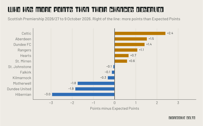
Celtic have about 2.4 more points than their chances deserved; Hibs are 3.0 short. A big +/− isn’t proof of luck on its own. Some teams may sit in a model blindspot, perhaps creating chances in situations that current xG models undervalue, but (over a large enough sample) most of it tends to even out.

However, in a season, we do not have infinite games to allow our sample to grow. We have 38. So, we need to ask: does xPoints actually predict final points at any stage?

To check, we split every Scottish Premiership season in half and compared each team’s first-half numbers with how many points per game it took in the second half. If xPoints is capturing anything worthwhile, it should be more informative than just points at this.

It is. First-half xPoints per game had a correlation of 0.81 with second-half points per game, against 0.74 for first-half actual points.

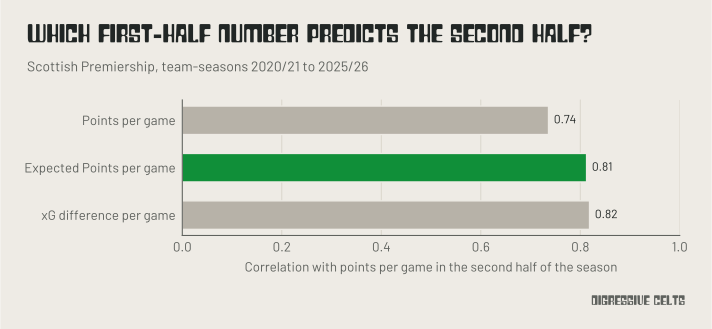
At this stage (19 games), Expected Goal Difference does just as well (0.82), and actual points aren’t miles behind. Earlier in the season, however, it is useful to have a common scale for our expected metrics where outliers are more impactful as they make a larger proportion of the whole.

Football is chaotic. xPoints gives us an indication of what was most likely to happen in a match given the chances that occurred. This gives us a better idea of what’s likely to happen later in the season.

References

Expected Goals

[1] Mead J, O’Hare A, McMenemy P (2023). Expected goals in football: improving model performance and demonstrating value. PLOS ONE, 18(4), e0282295. https://doi.org/10.1371/journal.pone.0282295

Modelling goals

[2] Maher MJ (1982). Modelling association football scores. Statistica Neerlandica, 36(3), 109–118. https://doi.org/10.1111/j.1467-9574.1982.tb00782.x

[3] Constantinou AC, Fenton NE (2012). Solving the problem of inadequate scoring rules for assessing probabilistic football forecast models. Journal of Quantitative Analysis in Sports, 8(1). https://doi.org/10.1515/1559-0410.1418

[4] Dixon MJ, Coles SG (1997). Modelling association football scores and inefficiencies in the football betting market. Journal of the Royal Statistical Society: Series C (Applied Statistics), 46(2), 265–280. https://doi.org/10.1111/1467-9876.00065

Appendix A: the exact calculation

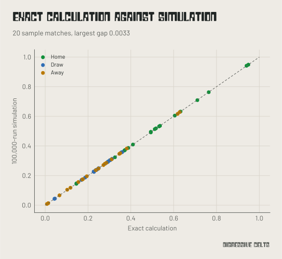
For each team, start with no shots taken: a 100% chance of no goals. Then add the shots one at a time. After a shot with an xG of p, the chance of the team having k goals becomes its chance of having k goals before that shot multiplied by (1 − p), plus its chance of having k − 1 goals before that shot multiplied by p. Once every shot is added, you have the exact chance of each number of goals (this is called a Poisson binomial distribution).

Combining the two teams is then simple. The chance of a home win is the total chance of every score where the home team has more goals than the away team, and likewise for draws and away wins.

This matches a simulation basically exactly (except simulation noise); see below.

Appendix B: the draw boost

The graph below shows the ranked probability score (top) and the predicted share of draws (bottom) for different multipliers on the chance of a draw, across every Scottish Premiership match from 2020/21 to 2025/26. With no boost, the method predicts too few draws. The best score comes at 1.060, and predicted draws match actual draws at around 1.04. We use 1.075, between the Scottish Premiership’s best value and the Premier League’s (1.090).

The extra chance of a draw is taken from each team in proportion to its chance of winning, so the probabilities still add up to one and the better team remains more likely to win. Refitting the multiplier with each season left out did slightly worse than keeping it fixed: the fitted value ranged from 1.02 to 1.14 depending on which season was left out, which is mostly noise.

Appendix C: how we tested the methods

Every method gave a probability of a home win, a draw, and an away win for each match, using only data from that match. Methods with something to fit (the draw multiplier, the Dixon–Coles adjustment, the xG difference model, and the machine-learning models) were fitted on all seasons but one and scored on the season left out, repeated for every season. We scored them with the ranked probability score, log loss, and the Brier score, which agreed, and compared methods match by match with bootstrap intervals. The Premier League (2020/21 to 2025/26) told the same story throughout.

The shot simulation is also well calibrated. Grouping matches by the predicted chance of each outcome, home wins, draws, and away wins all happened about as often as predicted:

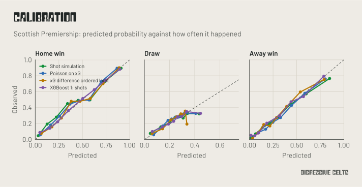
The machine-learning models were calibrated XGBoost models given five growing sets of match statistics: (1) xG in open play, from set plays, and in total, shots, shots inside and outside the box, and big chances; (2) plus possession, passes, passes in the opposition half, touches in the box, corners, crosses, long balls, dribbles, and offsides; (3) plus tackles, interceptions, clearances, duels, and aerials won; (4) plus shots on and off target, xG on target, blocked shots, big chances missed, and hitting the woodwork; and (5) plus saves, cards, and fouls. In set 3, both teams’ clearances were more important to the model than either team’s xG.

Appendix D: the ± ranges

For each team, we take its Expected Points from every match so far, resample them with replacement 1,000 times, add up each resample, and take the middle 95% of those totals. The ± shown is half the width of that range. The resampling uses a fixed random seed, so the numbers don’t jump around between updates. Dragging the date range on the standings page reruns the same calculation for just the matches in that range.